Chapter 1 Introduction
To begin with, we’ll focus on getting you started in R. We’ll look into installing our two key programs, R and RStudio. After that, we’ll look into how R can communicate with files on your system. Finally, we’ll look at the core packages for this course, how to do basic data manipulation using base R (R Core Team 2022), and tips for good practice when working with R. We’ll complete some exercises at the end so you can get a handle of the key concepts introduced here.
1.1 Installation and Setup
To get started, at the very least you’ll have to download R from CRAN. Select the correct distribution for your operating system and then click through to install R for the first time.
For Windows users, you’ll see a new page; at the top click on “Download R [version number] for Windows.” Click on that and follow the prompts in the installer. If you have a 64 bit system, install the 64 bit version of R as you’ll be able to take advantage of having more than 4Gb RAM. (This is useful in instances where you’re working with very large data sets.)
In R, you don’t want to type commands directly to the console. Instead, you should use a text editor to write your script and send it to the console as and when you want. This way, you’ll have a document of what you did, and any minor changes you have to make are very easy to implement (vs. writing it all out from scratch again).
One of the most popular ways to work on your R scripts is to use an Integrated Development Environment (IDE). The most popular IDE for R is RStudio, which you can download from the RStudio website. In the navigation panel, select products and choose RStudio. Scroll down until you see Download RStudio Desktop. Finally, for the Free tier, click the Download button and select the correct installer for your operating system. For Windows users, you should select RStudio [version number] - Windows Vista/7/8/10. Follow the prompts on the installer, and your system should automatically pick up that you already have R on your system. From there, be sure to open the RStudio program to get started. This is the logo that looks like this:
The RStudio logo
Once open, you’ll see something that should look like this. Only, you won’t have the top pane unless you choose to start a new script (File, New File, R script) or if you’ve opened an existing script already.
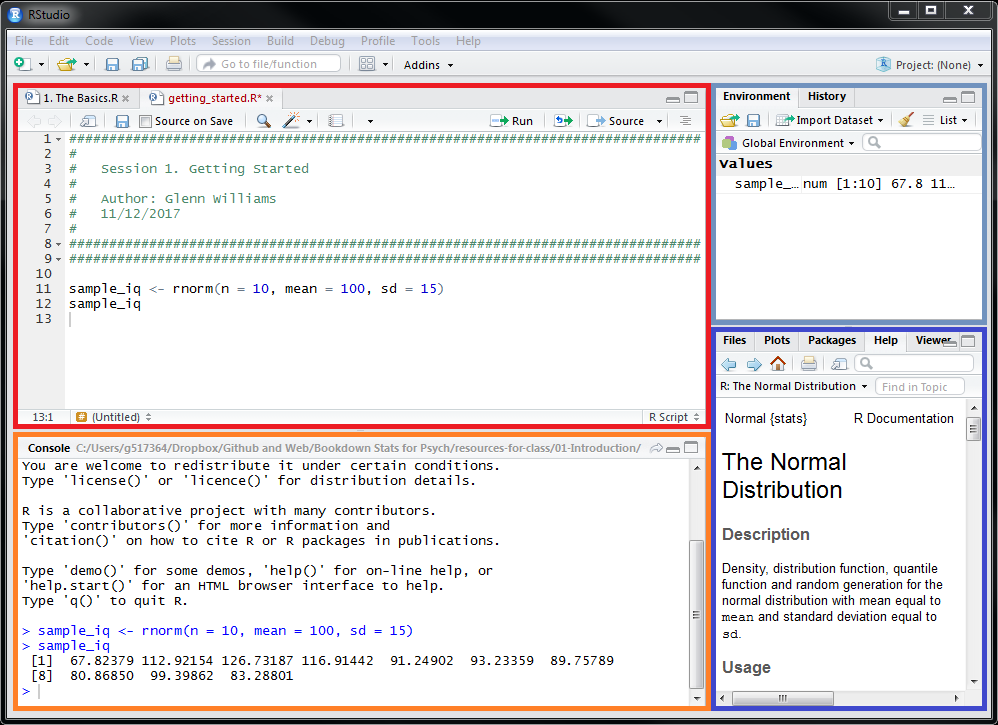
RStudio can be split into 4 main panes:
- The editor: Type, edit, and save scripts as you would in any text editor.
- The console: Execute scripts by typing and pressing enter.
- The environment and history: View objects (e.g. values, variables, and user-defined functions etc.) stored in memory for this working session. You can also see a history of your commands in the History tab.
- The viewer: view any files in your working directory, see your last plot from this session, view installed packages on your machine (you can also load them here), view the help documentation for any R commands, in the viewer you can view (surprise, surprise) markdown/other documents.
All of these panes are very useful when developing your R scripts, but RStudio has some other features such as syntax highlighting, code completion, and an easy interface for compiling your reproducible R-markdown notebooks. For advanced users, you can also set up projects that play nicely with Github for version control of your work.
Finally, RStudio defaults to giving you the option to save your workspace (e.g. all of the data you’ve created) when you close the program and to restore this workspace once you restart RStudio. I’d advise you to change RStudio’s defaults to never do this as this could cause unforseen errors when, for example, you want to change parts of script and you accidentally delete the stage to create a variable that is crucial later on. This deletion may not be obvious if you reload your workspace, but you won’t have a record of how you created said variable. To make these changes, go to Tools, Global Options then deselect Restore .RData into workspace at startup and from the dropdown menu on Save workspace to .RData on exit: to Never.
1.2 Working Directory and File Paths
When you create an R file (File, New File, R Script), where that file sits is its working directory. This is where R interprets any commands that go outside of your R session. For example, if you want to read data into R, or output a graph, R will do so in respect to the working directory. You can get your working directory like so:
getwd()You should see something along the lines of “C:/Users/YOUR_NAME/FOLDER/RFILE.R”
Now, you can set your working directory to any folder on your computer with an absolute file path. Often, people use absolute file paths in order read inputs and send outputs to different folders on their computer, telling R exactly where to look.
However, I recommend against this. That’s because if you change computers or pass your code over to someone else R will kick out an error saying it can’t find that folder; other computers are highly unlikely to have the same folder structure or even username as you, and fixing this can be frustrating. Also, it can be a pain having to type out your full file path, so let’s avoid that. Below, I’ve outlined one method for working that will allow you to use relative filepaths (relatively) easily.
If you want to keep your folder from getting cluttered, keep your R script(s) in a folder, with an Inputs and Outputs folder at that same level, like so:
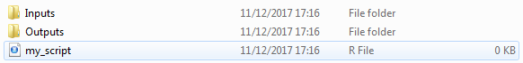
Potential Folder Structure for Your Projects
This way, when you want to read in raw data, or output a graph (or something else) you can use a relative file path rather than an absolute file path to define where your files are taken from/should go. This saves you a lot of typing of file paths, and it means your R scripts will work on someone else’s computer if you just send the entire folder containing the R script, Inputs, and Outputs folders.
To read in or save data using a relative file path, do this:
# reads a CSV file from the Inputs folder
my_data <- read.csv("Inputs/my_data.csv")

# writes a CSV file to the Outputs folder
my_data <- write.csv(my_data, "Outputs/my_data_again.csv")
You just have to type in the folder name and a slash (to indicate to go below that folder) and the name of your data. This saves you from all of the hassle of using an abosolute file path described above.
1.3 Packages
Next, while you can do a lot in base R, if you can think of some task that is reasonably laborious there’s probably a package out there that can help you to achieve a certain goal. For us, the whole data processing, analysis, and presentation workflow can be made so much simpler by using a set of packages from the tidyverse library (Wickham 2017). This package is required for what we’re about to do next, so install tidyverse (using install.packages("tidyverse")). Once installed, you needn’t do it again. But on each new session you have to define which packages you want to load into R using the library() command. Make sure to uncomment the install.packages("tidyverse") line if you haven’t installed this package yet.
# install.packages("tidyverse") # do this only once to install the package
library(tidyverse) # do this to load your package every time you open R
## ── Attaching packages ─────────────────────────────────────── tidyverse 1.3.2 ──
## ✔ ggplot2 3.3.6 ✔ purrr 0.3.4
## ✔ tibble 3.1.8 ✔ dplyr 1.0.10
## ✔ tidyr 1.2.1 ✔ stringr 1.4.1
## ✔ readr 2.1.2 ✔ forcats 0.5.2
## ── Conflicts ────────────────────────────────────────── tidyverse_conflicts() ──
## ✖ dplyr::filter() masks stats::filter()
## ✖ dplyr::lag() masks stats::lag()By default, R installs packages from CRAN, which is essentially a centralised network for all things R. However, some useful packages may not have been submitted here, and you can install them from other places, like GitHub. We won’t install packages from github or other repositories in this course. But it’s worth knowing that you can install packages from just about anywhere!
Most of the time, you won’t have any trouble using functions from a loaded package. However, there can be cases when you have two packages installed that use the same function name. To tell R exactly which version of a function to use, we can specify both the package and function name in the form package::function_name(). For example, we can use the group_by() function from the package dplyr by typing dplyr::group_by(). You won’t come across this in this course, as we’ll be using packages that have functions with unique names, but it’s worth bearing in mind if you come across problems with functions you know should work in the future.
Note: You may notice that in my code chunks I have some green text following a #. These are comments in R and are not read when you execute your code. Comments are very useful for telling you what each section of your code does, and how. I tend to comment quite heavily, as there’s always a chance you’ll forget what you’ve done when you go back to it after a few months away from the code.
1.4 Objects and Functions
You can use R like a calculator, e.g.
1 + 4## [1] 5You can execute this directly in the console, or run it from your R script by selecting that line of code (or highlighting several lines) and pressing Ctrl + Enter (for mac, this is probably Cmd + Enter). While I said you shouldn’t use the console when writing scripts, you can use it to test out a bit of code, or to quickly use R as a calculator when you’re in a meeting and feeling like mental arithmetic is a step too far. You can see that once the code is run, the R console returns the result back to you. You see a history of what you asked, and what was returned.
Top tip: use the up arrow key from the console and R will automatically fill in the last line/block of code you ran. Press up again to cycle back to older inputs, and down to back to the most recent ones.
R always waits for you to finish an expression before it runs your code. So, if you ended your line with a +, it’ll wait for the next number. This is useful for complex expressions that can take up multiple lines, e.g.
1 + 2 + 3 + 4 + 5 + 6 + 7 +
  8 + 9
## [1] 45Watch the console when you type this out. You’ll notice that if you press enter after typing 7 + on the new line you will no longer see > but you’ll see +. The same happens even if you pass a different mathematical operator (e.g. -, %, ^). This is there to tell you that R is not waiting for a new statement, but is waiting for you to finish off the current statement. If you see > it means that whatever you can start a new statement.
R also parses text if included in quotes. The same rule applies about finishing expressions here; if you don’t close your quote, then R will wait for you to do so. This means you can spread your text over several lines (by pressing Enter) and R will parse that as one expression. Note with our output we get \n which indicates that a new line follows the comma.
"Hello, world!"## [1] "Hello, world!""How are you doing today?
Things certainly have been interesting these past few years."## [1] "How are you doing today? \nThings certainly have been interesting these past few years."Crucially, you can store this sort of information in a variable. Variables are useful because you may want to use the results of a calculation and do some further operations on that result. This is especially useful if you’re not sure what that first result could be. We assign values to a variable using the assignment operator <- (read this as create from).
summed_numbers <- 5 + 8We can then output this variable later on, like so: (This is often useful for checking that your variables store what you think they store.)
summed_numbers## [1] 13Or we can perform operations on the variable.
summed_numbers*5## [1] 65Note: You cannot start variables with a number, you cannot use special characters (e.g. %!*) and you cannot include spaces in your variable name. Also, note that your capitalisation matters, so Summed_numbers is not summed_numbers. (I often get errors due to this issue…)
R has the simple arithmetic operations you’d expect from any program. For example, you can:
- add
x + y, - subtract
x - y, - multiply
x * y - divide
x/y, - exponentiate
x^y - find the modulus
x %% y, (e.g. 5 mod 2 = 1; i.e. the remainder from how many times 2 goes into 5) - and conduct integer division
x %/% y(e.g. 5 int div 2 = 2)
R also has some logical operations built in. For example:
- less than
x < y - less than or equal to
x <= y - greater than
x > y - greater than or equal to
x >= y - exactly equal to
x == y - not equal to
x != y - not x
!x - x OR y
x | y - x AND y
x & y - test if X is true
isTRUE(x)
These come in pretty handy for performing most operations on our data. If you’re unfamiliar with these, don’t worry. We’ll cover how you might use some of these in a staggered format as you progress through this course. Nicely, R also has a number of functions built in. This means you don’t need to write your own function if you want to sum a sequence of numbers. I’m sure I couldn’t provide an exhaustive list here, but as stated above we’ll cover most of the common functions as you get to grips with some data. Still, lets get an idea of how these functions work.
Below, we will sum the numbers 1 to 4. This function is built into R already, so we don’t have to write a whole lot of code for this.
sum(1, 2, 3, 4)## [1] 10What if we want to calculate the mean score from this set of numbers? That’s also built into R.
mean(1, 2, 3, 4)## [1] 1Notice that whenever we want to run a function, these functions always have a name and are followed by parentheses (e.g. mean(), sum()). What goes in the parentheses? The argument you want to pass to the function. These can have default values, or not (requiring you to specify the argument). Above, we passed the values 1 through 4 as the arguments to the mean() function. Later, we’ll look at functions that ask for arguments from separate data types (e.g. numbers and characters). If you’re unsure what an argument does, you can always ask R what it does, how it does it, and what to pass to it by using ?, e.g. ?mean(). This will bring up a document in the Help window of RStudio.
Typing out all of these numbers each time we want to perform some operation is a little tedious. To fix this, we can use what we learned above and store these numbers into a variable. In order to save these into their own variable, we use the c function. Think of this as concatenation. When we combine values into a variable, this variable is stored in our global environment. This means that we can perform operations on the variable later on, without the worry of typing our the values again. This is particularly useful if you want to store values from one function (say a statistical test) that you cannot pre-define but that you want to use later on.
Let’s give that a go. First, we’ll concatenate our values into a variable using the c() function described above. Here, we simply define that we want to concatenate some values, and list each value separated by a comma.
stored_values <- c(1, 2, 3, 4)If we then call a function that works with a set of numbers, it should also work if we call that function on the variable storing those numbers. Let’s see how this works with the mean() function.
mean(stored_values)## [1] 2.5Great! That’ll save is a lot of time writing and rewriting code later on. This also allows our code to be flexible, in that we can write a script that performs operations on variables that can take any range of values. This, to me, is one of the nicest things about doing your analyses in R. While you may spend more time getting your script up and running in the first place when compared to using point-and-click methods (e.g. in SPSS), if you gain new data or run a new experiment, it’s likely that your script can simply be re-run with no (or few) changes at very little cost to your time.
Now, this part is pretty important but may only be obvious if you’ve programmed in other languages. R is a vectorised language, which means that, as with the sum() function above, R can perform operations on the entire variable So, if you want to increment all values in your variable by 1, you can simply tell R to do so in one line of code, without the need for loops or other complex methods.
stored_values + 1## [1] 2 3 4 51.5 Creating and Accessing Data
So, you’ve made it through all of the boring stuff. Now we can look at manipulating some data in R.
Let’s pretend we’ve administered IQ tests to 100 participants. For some reason, we’re interested in whether dog and cat owners have different IQs. I’m sure some of you can come up with some incredibly biased hypotheses here, but we’ll leave that out for now.
We’ll create this data in R, then take a look at it using some of the packages from the tidyverse library that you installed and loaded above. If the functions below don’t work, be sure to load the tidyverse library (using library(tidyverse)) before running the code below.
First, we’ll create a variable containing the numbers 1 to 100, using the seq() function; this can be our participant ID variable. Next, we’ll use the sample() function to sample randomly (and with replacement) from the two labels “cat” and “dog” which acts as our factor for pet ownership. (Note that here I use the sample() function on the concatenated values of “cat” and “dog”, but this would work equally well with a variable containing these labels.) Finally, we’ll use the rnorm() function to generate some random numbers (sampled from the normal distribution) with a mean of 150, and a standard deviation of 15 to act as our IQ scores.
Remember how I said we’d look at functions that take several arguments? Well, thats what all of these functions below do. We define each parameter of the argument within the function call. So, if we want to generate a sequence of numbers from 1 to 100 , in increments of 1s (e.g. seq(from = 1, to = 100, by = 1)), then we define each argument with its name (e.g. from/to/by) and tell R which values to set for these arguments using =.
# create participant IDs
participant <- seq(from = 1, to = 100, by = 1)

# create pet ownership codes
set.seed(88)
pet <- sample(c("cat", "dog"), 100, replace = TRUE)

# create IQ scores
set.seed(88)
IQ_score <- rnorm(n = 100, mean = 150, sd = 15)
IQ_score <- round(IQ_score) # round IQ scores
Note: I’ve overspecified the functions above. You can simply run seq(1: 100) and rnorm(100, 150, 15) to get the same results, but it’s a little less readable. Here, and throughout, I’ll use the most readable version so you have the best idea of what you’re doing. Because we’re using random sampling, I’ve also set a seed, so that you’ll sample the same values as me. If you want people to be able to reproduce your random sampling so they get the same data, set a seed!
Finally, it’s important to note that you can call a function on the result of another function in R.
Right now, each number in the participant variable is unique. We can see how many participants are in the study by asking R “how long is the variable, participant?”. We do this like so:
length(participant)## [1] 100Cool, we have 100 participants! But what if we have several observations for one participant? I’ll define that (very simply) in the code below:
participant[2] <- 1 # assign the second value of participant the integer 1
head(participant) # return the first 6 values of the participant variable
## [1] 1 1 3 4 5 6Now, using length(participant) will return 100, because there’s still 100 values in the participant variable. How do we find how many unique numbers are in the participant variable? We simply nest the unique() function within the length() function:
length(unique(participant))## [1] 99This asks R how many unique values are in the variable participant. That’s 99!
1.5.0.1 Data Frames and Tibbles
Now, in the real world, if you tested IQs you’d typically have this data stored in a table somewhere prior to reading it into R. So lets pair the data together into a table in R. The most useful way to do this is to create a data.frame. But, since we’ve already loaded the tidyverse, we may as well use the built in tibbles. These are like data frames, but they have some different defaults that make working in the tidyverse easier.
IQ_data <- tibble::tibble(
  participant_number = participant,
  pet_id = pet,
  IQ = IQ_score
  )
What’s the main advantage of using a tibble over a data.frame here? Tibbles don’t automatically convert certain data types. With data.frame, character data is automatically converted to a factor. This can be useful, but not always. The thing I like most is that tibbles show the data type under the column name. This is taken from str() which tells you the structure of your data. Also, tibbles default to printing the first 10 rows of data when you type their name in the console. This will stop you from getting overwhelmed by a massive printout if you have a lot of data. Let’s see all of this in action.
IQ_data## # A tibble: 100 × 3
## participant_number pet_id IQ
## <dbl> <chr> <dbl>
## 1 1 cat 147
## 2 1 cat 160
## 3 3 dog 185
## 4 4 cat 122
## 5 5 cat 157
## 6 6 dog 152
## 7 7 cat 152
## 8 8 cat 119
## 9 9 cat 131
## 10 10 dog 160
## # … with 90 more rowsIf you want more than 10 rows, or a specific number of columns, tell R that’s what you’d like. Here, we’ve asked for the first 12 rows, and the width of the table to be infinity so that R prints out all columns even if they don’t fit on 1 row in the console. However, with only 3 columns, that isn’t an issue here.
print(IQ_data, n = 12, width = Inf)## # A tibble: 100 × 3
## participant_number pet_id IQ
## <dbl> <chr> <dbl>
## 1 1 cat 147
## 2 1 cat 160
## 3 3 dog 185
## 4 4 cat 122
## 5 5 cat 157
## 6 6 dog 152
## 7 7 cat 152
## 8 8 cat 119
## 9 9 cat 131
## 10 10 dog 160
## 11 11 cat 138
## 12 12 dog 165
## # … with 88 more rowsUnfortunately, some older functions in R won’t allow you to use a tibble. If this is the case, simply convert your tibble to a data.frame using the as.data.frame() function. Note, we use head() to see the head of our data frame, or the first 6 values. This is necessary here to avoid printing out each row, as we’re not in using a tibble any more. Notice that We’ve assigned the data.frame version of our IQ data to a new variable, rather than overwriting the previous variable. This is good practice when testing your code, as you never know what might break, resulting in data loss. (Although this wansn’t strictly necessary here.)
IQ_data_df <- as.data.frame(IQ_data)
head(IQ_data_df)
## participant_number pet_id IQ
## 1 1 cat 147
## 2 1 cat 160
## 3 3 dog 185
## 4 4 cat 122
## 5 5 cat 157
## 6 6 dog 1521.5.0.2 Accessing Tibble Information
With tibbles and data.frames, you often want to access a specific column in order to perform some calculation. Let’s say we want to calculate the mean IQ score in our data set. Why doesn’t the code below work?
mean(IQ_data)## Warning in mean.default(IQ_data): argument is not numeric or logical: returning
## NA## [1] NAR gives us a warning, saying that the argument to our function (i.e. the tibble, IQ_data) is not numeric or logical. Therefore, R cannot calculate the mean on something that isn’t a number (or set of numbers). Instead, we have to point R to the correct column within the tibble. This is often done by name using $ , or by name/position in the tibble using [[ and the name/position followed by ]].
First, let’s see that we’re accessing everything correctly here.
# by name
IQ_data$IQ
IQ_data[["IQ"]]

# by position
IQ_data[[3]]
## [1] 147 160 185 122 157 152Tibbles are stricter than data frames, in that they’ll always return a tibble. For example, with a data.frame if you ask for a value in a specific row of a specific column under the format data_frame[row, column], R will return a vector of the value at that position in the data.frame. With tibbles, your single value will be returned as a tibble.
# tibble output
IQ_data[1, 3] # row 1, col 3
## # A tibble: 1 × 1
## IQ
## <dbl>
## 1 147# data.frame output
IQ_data_df[1, 3]## [1] 147Now, lets calculate the mean on the correct column in the tibble. Personally, I prefer using $ for cases like this. But, feel free to use any of the above methods.
mean(IQ_data$IQ)## [1] 150.17We can combine what we learned above about c() to access multiple columns at once:
IQ_data[, c("participant_number", "IQ")]## # A tibble: 100 × 2
## participant_number IQ
## <dbl> <dbl>
## 1 1 147
## 2 1 160
## 3 3 185
## 4 4 122
## 5 5 157
## 6 6 152
## 7 7 152
## 8 8 119
## 9 9 131
## 10 10 160
## # … with 90 more rowsOr we can access a range of values by specifying the rows we’d like to access:
IQ_data[c(1, 2, 3, 4, 5), c("participant_number", "IQ")]## # A tibble: 5 × 2
## participant_number IQ
## <dbl> <dbl>
## 1 1 147
## 2 1 160
## 3 3 185
## 4 4 122
## 5 5 157or, to save typing, we can just define this from a starting to an ending value for the rows:
IQ_data[1:5, c("participant_number", "IQ")]## # A tibble: 5 × 2
## participant_number IQ
## <dbl> <dbl>
## 1 1 147
## 2 1 160
## 3 3 185
## 4 4 122
## 5 5 157In Session 4 we’ll look at more intuitive ways of accessing data from columns and rows in your data frames. However, for now we’ll quickly look at ways to manipulate data using the base R functionality so you have some idea how indexing works in R.
1.5.0.3 Manipulating Tibble Information
1.5.0.3.1 Changing Values
We can use these same principles to edit the information within our data. Say, we’d like to change participant number in row 2 back to 2, we just need to do this:
# specifying row and column by index
IQ_data[2, 1] <- 2

# specifying row by index and column by name
IQ_data[2, "participant_number"] <- 2

# specifying index within a column
IQ_data$participant_number[2] <- 2
You can see how all of this combined can result in some pretty powerful flexibility in how you access and manipulate your data in R.
1.5.0.3.2 Adding and Removing Columns
To add a row to a data frame, we simply need to specify what we want to add and assign it a new name. Let’s say that we want to add a column that indicates the operating system used by each participant.
We may have this because we made assumptions that people who use Windows, macOS, or the Linux families of operating systems differ in their IQ. This is a silly example for several reasons, not only because you can use more than one system; but we’ll stick with this for now.
Imagine we already have a sample of operating systems to draw from. You don’t need to understand how this works, but briefly I’ve used the inbuilt sample() function to pick from the three names with replacement, skewing the probabilities to select windows most often, followed by mac, then linux. All that matters is that we’re assigning 100 names to a variable.
set.seed(1000) # make the sampling procedure the same for us all

operating_system <- sample(c("windows", "mac", "linux"),
                           size = 100,
                           replace = TRUE,
                           prob = c(0.5, 0.3, 0.2)
                           )
In the IQ_data set, we can add a new column for the operating systems used by the participants like so:
IQ_data$operating_system <- operating_system # add new column

head(IQ_data) # view first 6 rows
## # A tibble: 6 × 4
## participant_number pet_id IQ operating_system
## <dbl> <chr> <dbl> <chr>
## 1 1 cat 147 windows
## 2 2 cat 160 mac
## 3 3 dog 185 windows
## 4 4 cat 122 mac
## 5 5 cat 157 mac
## 6 6 dog 152 windowsNote that you can rename the column to anything you like. But, for consistency, I like to keep the same name as the variable which acts as the data source.
Finally, we can remove the new column (and any column) by setting the entire column to nothing (NULL), like so:
IQ_data$operating_system <- NULL # remove new column

head(IQ_data) # view first 6 rows
## # A tibble: 6 × 3
## participant_number pet_id IQ
## <dbl> <chr> <dbl>
## 1 1 cat 147
## 2 2 cat 160
## 3 3 dog 185
## 4 4 cat 122
## 5 5 cat 157
## 6 6 dog 152Now the data is back to its original format.
We’ll look at another way to remove one or several columns from your data frame in Session 4, but for now this a quick way to get things done using base R.
1.5.0.3.3 Adding and Removing Rows
What if we want to add a new row to our data? This may be less common than adding a new column for data processing purposes, but it’s good to know anyway.
First, we need to know what should go in each cell. Remember that we have to keep the data square, so you can’t have missing values when you add a row. If you don’t have any data, you can just put NA (with no quotations) to keep the data square but to show that you don’t have any value for a given cell.
Let’s assume we want to add a new participant, 101, who has a dog but an unknown IQ. We must define a list of data where we assign values to the columns that match up with our IQ data column headings. We do this like so:
# add new row with values
IQ_data[101, ] <- list(participant_number = 101, pet_id = "dog", IQ = NA)

tail(IQ_data) # see last 6 rows
## # A tibble: 6 × 3
## participant_number pet_id IQ
## <dbl> <chr> <dbl>
## 1 96 dog 148
## 2 97 dog 178
## 3 98 cat 156
## 4 99 dog 165
## 5 100 cat 150
## 6 101 dog NAHere, we have to define all our values to be added in parentheses, using the list() function:
- participant number is
101 - pet_id is
"dog" - IQ is
NA(i.e. unknown)
We then assign this to our data frame using the assignment operator (<-).
We have to tell R where these values should go in our data frame. Because we’re adding a new row, we specify the data frame, with row 101, and all columns (remember, an empty value after the comma = all columns).
Note, this is a little more complicated than assigning a new row to our data in a data.frame, but makes us be more specific about what we are adding and where. For more details on lists, keep reading this section.
We can then remove this row again setting our data frame to itself, minus the 101st row:
IQ_data <- IQ_data[-101, ] # remove the new row

tail(IQ_data) # see last 6 rows
## # A tibble: 6 × 3
## participant_number pet_id IQ
## <dbl> <chr> <dbl>
## 1 95 dog 188
## 2 96 dog 148
## 3 97 dog 178
## 4 98 cat 156
## 5 99 dog 165
## 6 100 cat 150This is a pain as it isn’t consistent with removing the rows. But, in Session 4 we’ll look at removing rows in a consistent way to removing columns. Still, it’s useful to know how this process works.
1.5.0.4 Other Data Types
For most purposes, you’ll only need vectors and data frames/tibbles when you want to work with your data. But it’s worth being aware of other data types, such as lists and matrices.
With lists, you can define a vector that contains other objects. Think of this as nesting vectors within vectors (very meta).
person_quality <- list(glenn = c("handsome", "smart", "modest"),
                       not_glenn = c("less_handsome", "less_smart", "less_modest")
                       )
We can then access the elements of a list similarly to how we access vectors, but the name associated with the list will also be returned:
person_quality[1]## $glenn
## [1] "handsome" "smart" "modest"If, instead, we just want the values associated with that entry, we can use [[your list name]]:
person_quality[[1]]## [1] "handsome" "smart" "modest"We can edit these values in a similar way to how we did with a data frame. This time, we just need to tell R which vector to access first (here, it’s the first vector, using double brackets so we can access the values stored there, and not the name (as would happen if we just had 1 bracket)), and then specify which location in the vector you’d like to assign a new value using a separate bracket here:
person_quality[[1]][4] <- "liar"
person_quality[1]
## $glenn
## [1] "handsome" "smart" "modest" "liar"An advantage to using lists over data frames or tibbles is that the data need not be square. That is, you can have uneven lengths for your entries. Notice how glenn and not_glenn have different numbers of elements in the list. With a data frame, this is problematic. Let’s try adding another participant number to our IQ_data tibble.
IQ_data[101, 1] <- 101
tail(IQ_data)
## # A tibble: 6 × 3
## participant_number pet_id IQ
## <dbl> <chr> <dbl>
## 1 96 dog 148
## 2 97 dog 178
## 3 98 cat 156
## 4 99 dog 165
## 5 100 cat 150
## 6 101 <NA> NADid you notice that R automatically introduced NA values in the final cells for the pet_id and IQ columns?
Matrices work very similarly to data frames and tibbles, but they’re even stricter. They can only contain the same data type throughout, so we can’t mix columns containing characters and numbers without converting them all to the same data type (hint: it’s a character!). I’ll show you how to make a matrix, but we won’t linger on that as I haven’t found them all that useful in my own work.
matrix_example <- matrix(rep(1: 25),
                         nrow = 5,
                         ncol = 5
                         )
matrix_example
## [,1] [,2] [,3] [,4] [,5]
## [1,] 1 6 11 16 21
## [2,] 2 7 12 17 22
## [3,] 3 8 13 18 23
## [4,] 4 9 14 19 24
## [5,] 5 10 15 20 251.6 Good Practice
1.6.1 Data Checking Tips
Finally, a few tips on checking your data before you manipulate your data:
- If you’re unsure what you have in your working directory, use either check your environment (the panel in light blue in the RStudio screenshot above) or type
ls()in the console. This will list everything currently in the global environment. - If you want to know the data class for some object, use the
class()function (e.g.class(IQ_data)). - If you want to know the structure (including object classes) for some object, use the
str()function (e.g.str(IQ_data). Nicely,str()also tells you how many variables are in the object, and how many observations you have in total.
Most importantly with anything in R, if you aren’t sure how a function works, or what it’s done to your data, check how that function works! You can do this with any function by typing ? followed by the function name into the console (e.g. ?str()).
1.6.2 Style
I strongly recommend that you choose a style guide and stick to it throughout when you write your R code. This will make it easier to notice any errors in your code, and increases readability for you and others. Consistency is key here. Since we’re using a tidyverse first approach to teaching R in this course, I recommend this one by the creator of the tidyverse:
R Style Guide by Hadley Wickham
The important things to take home are that:
- Use sensible variable names: if a column shows, e.g. participant weight, call it participant_weight
- Use verbs to describe user-defined functions: if you write a function to make all the descriptive statistics you could ever want, call it something like make_descriptives()
- use a consistent style, like snake_case_here, or even camelCase, but don’t mix_snake_and_camelCase.
- comment your code with descriptions of why you’ve done something: you can often work out how you did it by following your code, but the why is easily lost!
1.7 Exercises
Try out the exercises below, we’ll cover these in the class with the solutions uploaded at the beginning of each session in a separate downloadable link. Try to solve these questions before resorting to the solutions. I’ll be there to help out where necessary. First, I want you to figure out why some code doesn’t work, then we’ll move on to you manipulating data.
For the opener, we’ll look at the basics of solving issues with your code.
1.7.1 Question 1
What’s wrong with the following code?
# create a sequence from 0 to 40 in intervals of 2
sequence < - seq(from = 0, to = 40, by = 2)
1.7.2 Question 2
Why doesn’t this return anything?
# draw 100 times from a uniform distribution between 1 and 10
uniform_distribution <- runif(n = 100, min = 1, max = 10)
uniform_distrbiution
Now, we’ll work with a data set. But I’d like you to produce it. We’ll break this down into steps for now.
1.7.3 Question 3
Lets pretend we have 100 participants. Create a variable that will store participant IDs. Their IDs can be anything you like, but some sort of logical numbering looks best.
Hint: seq() is your friend here!
1.7.4 Question 4
Create a variable that will store their scores on some test. Let’s assume participant scores are drawn from a normal distribution with a mean of 10 and an SD of 0.75.
Hint: rnorm() is a wonderful thing.
1.7.5 Question 5
Finally, create some ages for your participants. Here, you’ll have to use a new command called sample(). See if you can figure out how to use this command. If you’re lost, remember to use ? on the function.
1.7.6 Question 6
Create a data frame consisting of your participant IDs, their ages, and test scores.
1.7.7 Question 7
Take a look at the start and the end of your data frame. Do the values look reasonable? (Don’t worry about outliers or missing values etc., we’ll check those in later classes.)
1.7.8 Question 8
Access the row (and all columns) for participant 20. What do the scores look like? Are they the same as the person sitting next to you? Why or why not, might this be the case?
1.7.10 Question 10
Output some simple descriptive statistics from your sample. We want to know:
- Mean age
- Mean score
- SD score (Hint: Use
sd())
It may be useful to store these descriptives in another data frame for further use later on. Can you do that?